Synthetic control with pymc models#
import arviz as az

import causalpy as cp
%load_ext autoreload
%autoreload 2
%config InlineBackend.figure_format = 'retina'
seed = 42
Load data#
df = cp.load_data("sc")
treatment_time = 70
Run the analysis#
Note
The random_seed keyword argument for the PyMC sampler is not necessary. We use it here so that the results are reproducible.
df.head()
| a | b | c | d | e | f | g | counterfactual | causal effect | actual | |
|---|---|---|---|---|---|---|---|---|---|---|
| 0 | 0.793234 | 1.277264 | -0.055407 | -0.791535 | 1.075170 | 0.817384 | -2.607528 | 0.144888 | -0.0 | 0.398287 |
| 1 | 1.841898 | 1.185068 | -0.221424 | -1.430772 | 1.078303 | 0.890110 | -3.108099 | 0.601862 | -0.0 | 0.491644 |
| 2 | 2.867102 | 1.922957 | -0.153303 | -1.429027 | 1.432057 | 1.455499 | -3.149104 | 1.060285 | -0.0 | 1.232330 |
| 3 | 2.816255 | 2.424558 | 0.252894 | -1.260527 | 1.938960 | 2.088586 | -3.563201 | 1.520801 | -0.0 | 1.672995 |
| 4 | 3.865208 | 2.358650 | 0.311572 | -2.393438 | 1.977716 | 2.752152 | -3.515991 | 1.983661 | -0.0 | 1.775940 |
result = cp.SyntheticControl(
    df,
    treatment_time,
    control_units=["a", "b", "c", "d", "e", "f", "g"],
    treated_units=["actual"],
    model=cp.pymc_models.WeightedSumFitter(
        sample_kwargs={"target_accept": 0.95, "random_seed": seed}
    ),
)
Show code cell output
Initializing NUTS using jitter+adapt_diag...
Multiprocess sampling (4 chains in 4 jobs)
NUTS: [beta, y_hat_sigma]
Sampling 4 chains for 1_000 tune and 1_000 draw iterations (4_000 + 4_000 draws total) took 6 seconds.
Sampling: [beta, y_hat, y_hat_sigma]
Sampling: [y_hat]
Sampling: [y_hat]
Sampling: [y_hat]
Sampling: [y_hat]
fig, ax = result.plot(plot_predictors=True)
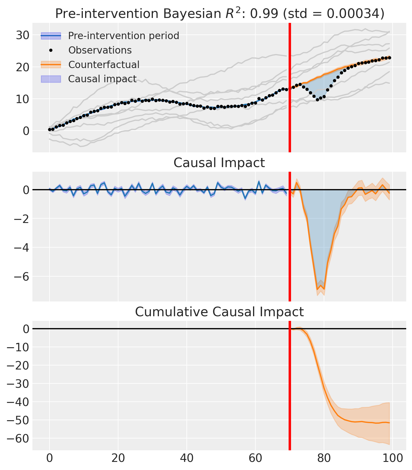
result.summary()
================================SyntheticControl================================
Control units: ['a', 'b', 'c', 'd', 'e', 'f', 'g']
Treated unit: actual
Model coefficients:
    a            0.33, 94% HDI [0.3, 0.38]
    b            0.05, 94% HDI [0.011, 0.089]
    c            0.3, 94% HDI [0.26, 0.35]
    d            0.054, 94% HDI [0.01, 0.1]
    e            0.024, 94% HDI [0.001, 0.065]
    f            0.2, 94% HDI [0.11, 0.26]
    g            0.038, 94% HDI [0.0028, 0.087]
    y_hat_sigma  0.26, 94% HDI [0.22, 0.31]
As well as the model coefficients, we might be interested in the average causal impact and average cumulative causal impact.
az.summary(result.post_impact.mean("obs_ind"))
| mean | sd | hdi_3% | hdi_97% | mcse_mean | mcse_sd | ess_bulk | ess_tail | r_hat | |
|---|---|---|---|---|---|---|---|---|---|
| x[actual] | -1.72 | 0.212 | -2.117 | -1.35 | 0.006 | 0.004 | 1152.0 | 1649.0 | 1.0 |
Warning
Care must be taken with the mean impact statistic. It only makes sense to use this statistic if it looks like the intervention had a lasting (and roughly constant) effect on the outcome variable. If the effect is transient, then clearly there will be a lot of post-intervention period where the impact of the intervention has ‘worn off’. If so, then it will be hard to interpret the mean impacts real meaning.
We can also ask for the summary statistics of the cumulative causal impact.
# get index of the final time point
index = result.post_impact_cumulative.obs_ind.max()
# grab the posterior distribution of the cumulative impact at this final time point
last_cumulative_estimate = result.post_impact_cumulative.sel({"obs_ind": index})
# get summary stats
az.summary(last_cumulative_estimate)
| mean | sd | hdi_3% | hdi_97% | mcse_mean | mcse_sd | ess_bulk | ess_tail | r_hat | |
|---|---|---|---|---|---|---|---|---|---|
| x[actual] | -51.61 | 6.35 | -63.52 | -40.51 | 0.186 | 0.105 | 1152.0 | 1649.0 | 1.0 |
Effect Summary Reporting#
For decision-making, you often need a concise summary of the causal effect with key statistics. The effect_summary() method provides a decision-ready report with average and cumulative effects, HDI intervals, tail probabilities, and relative effects.
# Generate effect summary for the full post-period
stats = result.effect_summary(treated_unit="actual")
stats.table
| mean | median | hdi_lower | hdi_upper | p_gt_0 | relative_mean | relative_hdi_lower | relative_hdi_upper | |
|---|---|---|---|---|---|---|---|---|
| average | -1.720330 | -1.705730 | -2.141285 | -1.344371 | 0.0 | -9.142522 | -11.144332 | -7.299538 |
| cumulative | -51.609893 | -51.171893 | -64.238552 | -40.331122 | 0.0 | -9.142522 | -11.144332 | -7.299538 |
print(stats.text)
Post-period (70 to 99), the average effect was -1.72 (95% HDI [-2.14, -1.34]), with a posterior probability of an increase of 0.000. The cumulative effect was -51.61 (95% HDI [-64.24, -40.33]); probability of an increase 0.000. Relative to the counterfactual, this equals -9.14% on average (95% HDI [-11.14%, -7.30%]).
You can customize the summary in several ways:
Window: Analyze a specific time period instead of the full post-period
Direction: Specify whether you’re testing for an increase, decrease, or two-sided effect
Options: Include/exclude cumulative or relative effects
# Example: Analyze first half of post-period
post_indices = result.datapost.index
window_start = post_indices[0]
window_end = post_indices[len(post_indices) // 2]

stats_windowed = result.effect_summary(
    window=(window_start, window_end),
    treated_unit="actual",
    direction="two-sided",
    cumulative=True,
    relative=True,
)

stats_windowed.table
| mean | median | hdi_lower | hdi_upper | p_two_sided | prob_of_effect | relative_mean | relative_hdi_lower | relative_hdi_upper | |
|---|---|---|---|---|---|---|---|---|---|
| average | -3.057512 | -3.045187 | -3.430665 | -2.706604 | 0.0 | 1.0 | -18.635032 | -20.456322 | -16.867122 |
| cumulative | -48.920194 | -48.722991 | -54.890645 | -43.305657 | 0.0 | 1.0 | -18.635032 | -20.456322 | -16.867122 |
print(stats_windowed.text)
Post-period (70 to 85), the average effect was -3.06 (95% HDI [-3.43, -2.71]), with a posterior probability of an effect of 1.000. The cumulative effect was -48.92 (95% HDI [-54.89, -43.31]); probability of an effect 1.000. Relative to the counterfactual, this equals -18.64% on average (95% HDI [-20.46%, -16.87%]).