Synthetic control with scikit-learn models

import causalpy as cp

Load data

df = cp.load_data("sc")
treatment_time = 70

Analyse with WeightedProportion model

result = cp.SyntheticControl(
    df,
    treatment_time,
    control_units=["a", "b", "c", "d", "e", "f", "g"],
    treated_units=["actual"],
    model=cp.skl_models.WeightedProportion(),
)

fig, ax = result.plot(plot_predictors=True)

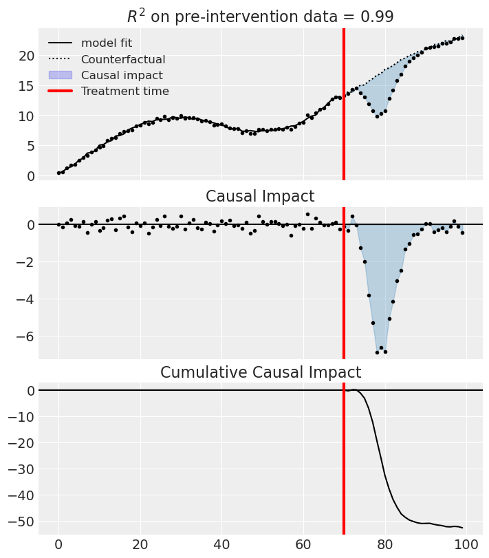
result.summary(round_to=3)

================================SyntheticControl================================
Control units: ['a', 'b', 'c', 'd', 'e', 'f', 'g']
Treated unit: actual
Model coefficients:
  a	     0.319
  b	    0.0597
  c	     0.294
  d	    0.0605
  e	  0.000762
  f	     0.234
  g	    0.0321

Effect Summary Reporting

For decision-making, you often need a concise summary of the causal effect. The effect_summary() method provides a decision-ready report with key statistics.

Note

OLS vs PyMC Models: When using OLS models (scikit-learn), the effect_summary() provides confidence intervals and p-values (frequentist inference), rather than the posterior distributions, HDI intervals, and tail probabilities provided by PyMC models (Bayesian inference). OLS tables include: mean, CI_lower, CI_upper, and p_value, but do not include median, tail probabilities (P(effect>0)), or ROPE probabilities.

# Generate effect summary for the full post-period
stats = result.effect_summary()
stats.table

	mean	ci_lower	ci_upper	p_value	relative_mean	relative_ci_lower	relative_ci_upper
average	-1.757497	-2.625051	-0.889943	0.000271	-10.132258	-15.262594	-5.001922
cumulative	-52.724907	-78.751527	-26.698286	0.000271	-303.967744	-457.877827	-150.057661

# View the prose summary
print(stats.text)

Post-period (70 to 99), the average effect was -1.76 (95% CI [-2.63, -0.89]), with a p-value of 0.000. The cumulative effect was -52.72 (95% CI [-78.75, -26.70]); p-value 0.000. Relative to the counterfactual, this equals -10.13% on average (95% CI [-15.26%, -5.00%]).

But we can see that (for this dataset) these estimates are quite bad. So we can lift the “sum to 1” assumption and instead use the LinearRegression model, but still constrain weights to be positive. Equally, you could experiment with the Ridge model (e.g. Ridge(positive=True, alpha=100)).